Huffman coding from scratch with Elixir
Huffman coding is a pretty straight-forward lossless compression algorithm first described in 1992 by David Huffman. It utilizes a binary tree as its base and it’s quite an easy to grasp algorithm. In this post we walk through implementing a Huffman coder and decoder from scratch using Elixir ⚗️
How does Huffman work?
In this example we assume the data we are compressing is a piece of text, as text lends itself very well for compression due to repetition of characters.
The algorithm in its core works by building a binary tree based on the frequency of the individual characters. Placing characters with a higher frequency closer to the root of the tree than characters with a lower one.
The Huffman code can be derived by walking the tree until we find the character. Every time we pick the left-child, we write down a 0 and for every right-child a 1. Repeat the process for each character in the text, and voila!
Decoding the text is as simple as starting at the root of the tree and traverse down the left-child for every 0 you encounter and pick the right-child for every 1. Once you hit a character, write it down and start over with the remainder of the bits.
For an excellent explanation on the Huffman Coding algorithm, give this explainer video by Tom Scott a watch!
Let’s get to work: Setting up the project
Ok! Let’s begin by generating a new Mix project using mix new huffman. cd huffman into the project root and open up the lib/huffman.ex file. This file contains our Huffman module. Replace the contents of the file with a single function declaration encode/1 like so:
1defmodule Huffman do
2  def encode(text \\ "cheesecake") do
3  end
4end
This function accepts the text we like to compress and defaults to “cheesecake” because, why not 🤷
Frequency analysis
The first step in Huffman coding is a simple frequency analysis. For each character in the given text, count how many times it is used in the text. This is a rather crucial part of the encoding algorithm as this determines where the characters are placed in the binary tree.
For example; when encoding the word “cheesecake” we can already see that certain characters appear more than others. e is used four times whereas the c appears only twice.
Let’s write some code that does the frequency analysis for us. Update our encode/1 function to match the following:
1def encode(text \\ "cheesecake") do
2  frequencies =
3    text
4    |> String.graphemes()
5    |> Enum.reduce(%{}, fn char, map ->
6      Map.update(map, char, 1, fn val -> val + 1 end)
7    end)
8end
This code above splits the input string into graphemes (individual characters) and stores the count per character in a map using Map.update/4.
Popping into an iex shell and running Huffman.encode now gives us the following output:
1%{
2  "a" => 1,
3  "c" => 2,
4  "e" => 4,
5  "h" => 1,
6  "k" => 1,
7  "s" => 1
8}
Sorting the characters
Since order is important when building our tree, we need to sort the list of characters by their frequency. Luckily Elixir’s Enum module comes to the rescue. Add the following code to our Huffman.encode/1 function:
1queue =
2  frequencies
3  |> Enum.sort_by(fn {_char, frequency} ->
4    frequency
5  end)
By passing the map with frequencies to Enum.sort_by/2, we sort the map using its values (the frequencies). This outputs:
1[
2  {"a", 1},
3  {"h", 1},
4  {"k", 1},
5  {"s", 1},
6  {"c", 2},
7  {"e", 4}
8]
Building the tree
Before we can neatly build a tree, we need to determine which kinds of nodes we have. We have a Leaf node which holds a single character and a Node which contains a left- and a right child. Each child on its own can be another Node or a Leaf.
Let’s define two structs to model these types of nodes at the top or our module:
1defmodule Node do
2  defstruct [:left, :right]
3end
4
5defmodule Leaf do
6  defstruct [:value]
7end
Note: Make sure you define the two structs within our current Huffman module to avoid naming clashes with the built-in Node.
The next step is to iterate over our list of sorted characters and convert them to Leaf nodes. Extend our Huffman.encode/1 function like this:
1  queue =
2    frequencies
3    |> Enum.sort_by(fn {_node, frequency} -> frequency end)
4+   |> Enum.map(fn {value, frequency} ->
5+        {
6+          %Leaf{value: value},
7+          frequency
8+        }
9+   end)
Now that we have an ordered set of Leaf nodes, we can build up the rest of the binary tree. Define a new function to do exactly this:
 1defp build([{root, _freq}]), do: root
 2
 3defp build(queue) do
 4  [{node_a, freq_a} | queue] = queue
 5  [{node_b, freq_b} | queue] = queue
 6
 7  new_node = %Node{
 8    left: node_a,
 9    right: node_b
10  }
11
12  total = freq_a + freq_b
13
14  queue = [{new_node, total}] ++ queue
15
16  queue
17  |> Enum.sort_by(fn {_node, frequency} -> frequency end)
18  |> build()
19end
Since this is a recursive function we need an exit condition, otherwise we are looping forever. In our case we are done building the tree when there is only a single root-node in the queue. The second clause is a bit more beefy, let’s break it down:
First thing we do is pop two nodes of the queue by pattern matching the tuple
{node, frequency}as the head of the list, and matching the rest of the list again asqueue. Doing this twice gives us two nodes and their frequencies we can work with.The next step is combining these two nodes in a parent
Nodeand tallying up the frequencies so we can prepend it to the queue.The next step is sorting the queue again to make sure the items with the lowest frequency are at the head of the queue.
The last step is to call
build/1again so this process starts all over again.
Calling our build/1 function at the end of our Huffman.encode/1 function passing the queue of items results in:
 1%Huffman.Node{
 2  left: %Huffman.Leaf{value: "e"},
 3  right: %Huffman.Node{
 4    left: %Huffman.Leaf{value: "c"},
 5    right: %Huffman.Node{
 6      left: %Huffman.Node{
 7        left: %Huffman.Leaf{value: "k"},
 8        right: %Huffman.Leaf{value: "s"}
 9      },
10      right: %Huffman.Node{
11        left: %Huffman.Leaf{value: "a"},
12        right: %Huffman.Leaf{value: "h"}
13      }
14    }
15  }
16}
The output above shows a tree structure where the character e is placed more towards the root of the tree and the character a is placed more towards the bottom. Each node in our tree is either a Leaf with the actual character or another Node. Drawn out this looks like:

Our Huffman tree
Encoding the text
Now that we have the Huffman tree all setup and ready to go, let’s focus on encoding the text using Huffman coding. The process of doing so is quite simple:
Look up each character of the text in our binary tree and keep track of each step while traversing down the tree. Each time we traverse down the left-child, write down a 0 and each time we traverse down the right-child write down a 1. Once we find the character in the tree, the path we wrote down is our Huffman code.
An example
So for example, in our tree above, the letter “c” has the code 10 since at the first node we take the right branch and then the left branch and voila. Similarly for the character “s” the code is 1101 since for the first two nodes, we take the right branch, then the left and lastly the right one again.
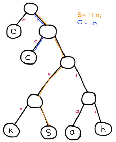
Encoding process of S an C
Code
First things first, we should be able to look up a character in the binary tree and keep track of its path while doing so.
 1defp find(tree, character, path \\ <<>>)
 2
 3defp find(%Leaf{value: value}, character, path) do
 4  case value do
 5    ^character -> path
 6    _ -> nil
 7  end
 8end
 9
10defp find(%Node{left: left, right: right}, character, path) do
11  find(left, character, <<path::bitstring, 0::size(1)>>) ||
12    find(right, character, <<path::bitstring, 1::size(1)>>)
13end
In the code example above we defined a function with two different clauses and a function header. The function header is just so that we can define a default value for the path which we set to an empty binary.
The first clause executes when passed in a Leaf node. The only thing we need to do is compare its value to the character we are looking for. When they match, return the path, else return nil.
The second clause matches on Nodes and calls find/3 with each child of the node, passing in an updated path. So when recursing on the left-child, we update the path with a 0. The || (or) operator makes sure that either of the two paths is returned.
Now that we can look up a single character in our binary tree, let’s iterate over all the characters in the text and replace them with their Huffman code. Add the following function to our Huffman module:
1defp convert(text, tree) do
2  text
3  |> String.graphemes()
4  |> Enum.reduce(<<>>, fn character, binary ->
5    code = find(tree, character)
6
7    <<binary::bitstring, code::bitstring>>
8  end)
9end
This function simply breaks the text into graphemes and iterates over each grapheme by calling Enum.reduce/3. Starting off with an empty binary, we can simply append to it for each character we find.
Now wire it all up and call our convert/2 function at the bottom of our Huffman.encode/1 function passing the original text and the tree.
The encode/1 function now looks like:
 1def encode(text \\ "cheesecake") do
 2  frequencies =
 3    text
 4    |> String.graphemes()
 5    |> Enum.reduce(%{}, fn char, map ->
 6      Map.update(map, char, 1, fn val -> val + 1 end)
 7    end)
 8
 9  queue =
10    frequencies
11    |> Enum.sort_by(fn {_node, frequency} -> frequency end)
12    |> Enum.map(fn {value, frequency} -> {%Leaf{value: value}, frequency} end)
13
14  tree = build(queue)
15  {tree, convert(text, tree)}
16end
As you can see it returns a tuple containing the tree and the encoded text. It returns the tree because we need this in the next step to decode the text to its original form again.
Calling Huffman.encode now results in the following:
 1{
 2  %Huffman.Node{
 3   left: %Huffman.Leaf{value: "e"},
 4   right: %Huffman.Node{
 5     left: %Huffman.Leaf{value: "c"},
 6     right: %Huffman.Node{
 7       left: %Huffman.Node{
 8         left: %Huffman.Leaf{value: "k"},
 9         right: %Huffman.Leaf{value: "s"}
10       },
11       right: %Huffman.Node{
12         left: %Huffman.Leaf{value: "a"},
13         right: %Huffman.Leaf{value: "h"}
14       }
15     }
16   }
17 }, <<188, 213, 216>>}
Where the second element of the tuple (<<188, 213, 216>>) is our compressed data.
Quick size comparison
1iex(1)> <<188, 213, 216>> |> bit_size()
224 # variable bit length per char, but max 4 bits in this scenario
3
4iex(2)> "cheesecake" |> bit_size()
580 # 10 chars * 8 bits per char = 80 bits
Using our Huffman module, encoding the string “cheesecake” results in a binary blob of only 24 bits. Each character in our binary tree is reachable in max. four steps, so each character is encoded in 4 bits or less. Using ASCII encoding each character takes 8 bits.
However, in order to decompress the text, we need access to the same tree we used to compress the text. Meaning that if we want to send the compressed data over the wire or store it to disk, we need need to account for additional space for the tree too.
Decoding
Now that we have coded ourselves the ability to encode text using Huffman coding, we also should have a way to decode the data back to its original form.
Decoding the data is quite straight-forward: all we need is our original Huffman tree and the encoded binary blob from the previous steps.
We use the binary blob as some sort of turn-by-turn navigation through our binary tree. From the top of the tree, traverse down the left-child when encountering a 0 in the data and traverse down the right-child when finding a 1.
Repeat this process until we hit a Leaf node. Write down the value of the Leaf and repeat with the remainder of the bits.
Code
First things first, we need a function that can walk the tree following the instructions in the compressed data, until we hit a Leaf node.
1defp walk(binary, %Leaf{value: value}), do: {binary, value}
2
3defp walk(<<0::size(1), rest::bitstring>>, %Node{left: left}) do
4  walk(rest, left)
5end
6
7defp walk(<<1::size(1), rest::bitstring>>, %Node{right: right}) do
8  walk(rest, right)
9end
In the code above we define a walk/2 function that takes the encoded binary and the tree and walks the tree. For every Node it encounters it looks at the next bit of the data to determine whether it should traverse down the first-child (found a 0) or traverse down the right-child (found a 1).
It keeps doing that until it finds a Leaf node, then it returns the remainder of the data and the character that belongs to that code.
Now that we have a function that can walk to the first available Leaf node following the instructions of the data, we want to call this function recursively as long as there’s more binary data available.
Let’s define another function:
1def decode(tree, data, result \\ [])
2
3def decode(_tree, <<>>, result),
4  do: List.to_string(result)
5
6def decode(tree, data, result) do
7  {rest, value} = walk(data, tree)
8  decode(tree, rest, result ++ [value])
9end
The decode/3 function above has two clauses. The last one basically walks the tree until it finds the first Leaf node, stores its character value in a list (result) and recurses with the remainder of the binary data.
The first clause matches once we have no binary data left to decode. It passes the result to List.to_string/1 concatenating the items in the list together forming a string.
The end result
That’s all there is to it! We built ourselves a Huffman Coder and Decoder using ~90 lines of Elixir:
 1defmodule Huffman do
 2  defmodule Node do
 3    defstruct [:left, :right]
 4  end
 5
 6  defmodule Leaf do
 7    defstruct [:value]
 8  end
 9
10  def encode(text \\ "cheesecake") do
11    frequencies =
12      text
13      |> String.graphemes()
14      |> Enum.reduce(%{}, fn char, map ->
15        Map.update(map, char, 1, fn val -> val + 1 end)
16      end)
17
18    queue =
19      frequencies
20      |> Enum.sort_by(fn {_node, frequency} -> frequency end)
21      |> Enum.map(fn {value, frequency} -> {%Leaf{value: value}, frequency} end)
22
23    tree = build(queue)
24    {tree, convert(text, tree)}
25  end
26
27  def decode(tree, data, result \\ [])
28
29  def decode(_tree, <<>>, result),
30    do: List.to_string(result)
31
32  def decode(tree, data, result) do
33    {rest, value} = walk(data, tree)
34    decode(tree, rest, result ++ [value])
35  end
36
37  defp walk(binary, %Leaf{value: value}), do: {binary, value}
38
39  defp walk(<<0::size(1), rest::bitstring>>, %Node{left: left}) do
40    walk(rest, left)
41  end
42
43  defp walk(<<1::size(1), rest::bitstring>>, %Node{right: right}) do
44    walk(rest, right)
45  end
46
47  defp build([{root, _freq}]), do: root
48
49  defp build(queue) do
50    [{node_a, freq_a} | queue] = queue
51    [{node_b, freq_b} | queue] = queue
52
53    new_node = %Node{
54      left: node_a,
55      right: node_b
56    }
57
58    total = freq_a + freq_b
59
60    queue = [{new_node, total}] ++ queue
61
62    queue
63    |> Enum.sort_by(fn {_node, frequency} -> frequency end)
64    |> build()
65  end
66
67  defp find(tree, character, path \\ <<>>)
68
69  defp find(%Leaf{value: value}, character, path) do
70    case value do
71      ^character -> path
72      _ -> nil
73    end
74  end
75
76  defp find(%Node{left: left, right: right}, character, path) do
77    find(left, character, <<path::bitstring, 0::size(1)>>) ||
78      find(right, character, <<path::bitstring, 1::size(1)>>)
79  end
80
81  defp convert(text, tree) do
82    text
83    |> String.graphemes()
84    |> Enum.reduce(<<>>, fn character, binary ->
85      code = find(tree, character)
86
87      <<binary::bitstring, code::bitstring>>
88    end)
89  end
90end
Next steps
There’s several improvements we can make to this implementation. For example, when encoding the text and looking up the Huffman code in the tree, we don’t have to walk the tree for every character. We can do a full traversal once and keep track of each character and its Huffman code in a map.
Also building up the queue can be improved. We don’t have to keep sorting the queue after every insert, rather have a look at a proper priority queue.
For an implementation that also serializes the tree to be written to disk or network, head over to the GitHub repository
Thanks for reading! 🤘